What is Expected Value?

Expected value refers to the anticipated value of a variable. It represents a generalization of the weighted average of a variable. Other names used for the expected value of a variable are expectation, mean, average, first moment, or mathematical expectation. While mostly associated with economics and statistics, the expected value is also crucial in finance and investing.

The calculation of expected value involves aggregating the product of the likelihood of an outcome occurring with each of the possible outcomes. For example, for four different outcomes, it is necessary to calculate what the probability of each outcome occurring is and then to multiply the product of those likelihoods with the outcomes. Then it is critical to sum all the results to get an expected value.

How does Expected Value apply in finance and investing?

In investing, investors usually use expected values to estimate a value for an investment in the future. For a random variable, its EV gives a measure of its center of the distribution. Similarly, calculating an expected value allows investors to evaluate various scenarios and choose the one most likely to achieve their desired output.

Therefore, it is a crucial concept used in scenario analysis, which is a technique for determining the expected value of an investment opportunity. Investors can not only calculate the expected value of single discrete variables but also for single continuous, multiple discrete, and multiple continuous variables. Therefore, it is also common to use expected values with multivariate models.

What is the formula for Expected Value?

The formula to calculate the expected value for a single event that repeats multiple times is straightforward, which is as below.

EV = P(X) x n

In the above formula, 'P(X)' represents the likelihood or probability of the event occurring, while 'n' shows the number of times the event will repeat. It is the simplest form of expected value. However, in investing, the calculations are more complicated and often involve multiple events. In these cases, the formula for expected value changes to compensate for multiple events, as below.

EV = ∑P(Xi) x Xi

In the above equation, ‘P(Xi)’ represents the probability of the event and ‘Xi’ denotes the event. However, the difference between the two formulas is that of the summation of expected values. In this case, investors must calculate various expected values for multiple events and aggregate them to get a probability-weighted average.

Example

An investor wants to decide between investing in two stocks. The first stock has a 60% chance of achieving a $1,000 return, while a 40% chance of getting a $500 return. On the other hand, the other stock has a 20% chance of a $2,000 return while an 80% chance of $400. To select the best option, the investor can calculate the expected value of both stocks and compare them with each other.

For the first stock, the expected value would be as follows.

EV = [60% x $1,000] + [40% x $500]

EV = $800

For the second stock, the expected value is as follows.

EV = [20% x $2,000] + [80% x $400]

EV = $640

According to the expected values of both stocks, the best option for the investor is to go with the first option.

Conclusion

Expected value is a concept used in statistics to represent the anticipated value of a variable. In finance and investing, it can help investors in estimating the value of an investment in the future. It is a concept that is the core of scenario analysis and multivariate models.

Originally Published Here: Formula for Expected Value

What is Median?

In mathematics, the median represents the middle point of a sorted list of numbers. In a way, it shows the average of a given set of numbers. For example, for a random set {12, 13, 18, 10, 5, 2, 9, 6, 15, 14, 3}, the median will be the number '10'. In order to find the median in the above set, it is necessary to sort the list first. The sorted list, in this case would be {2, 3, 5, 6, 9, 10, 12, 13, 14, 15, 18}.

From the sorted list given above, the median would represent its middle point. Since there are a total of 11 numbers in the list, the median would be the 6^th element of the list. In the sorted list, the 6^th element is the number '10'. Therefore, it is the median of that particular given set of numbers. As mentioned, however, the list must be sorted first.

The above set of numbers contains an odd number of elements. Therefore, the median for the list is only a single number. The number, in that case, '10', represents the central point of the sorted listed that has an equal number of elements above and below it. However, when a list contains an even number of elements, the median will be the average of the pair of numbers that fall in the middle.

Along with mean and mode, the median is a critical concept used to derive the average of a given set of data points. While the median represents the midpoint of the set, the mean and mode calculate the average differently. Another name used for the median is positional average, which gives an accurate description of what it is.

What are the uses of Median?

There are several uses of the median. Most commonly it can be used as a measure of location in cases where the extreme values of a given set of elements have low importance, usually due to a skewed distribution. Similarly, it helps when the extreme values of a set are unknown or when the anomalies or outliers are untrustworthy.

For example, in the set {5, 20, 22, 22, 23, 23, 43}, the mode is 22, which is a better representative of the positional average of the set. In the case of the given set, both the extreme ends (5 and 43) may represent extreme values that are untrustworthy due to how different they are from the average.

Similarly, the median is simple to understand and easy to calculate. However, that does not take away from its usefulness and application in mathematics and other fields. It is one of the most well-known summary statistics in descriptive statistics while also being a robust approximation to the mean.

Can Median help in finance and investing?

In finance and investing, the median can also have an application, especially during comparable analysis. When comparing between stocks of different nature, investors may want to neglect the extreme values that they consider untrustworthy or are significantly different from the average of the given data. In that case, using other ways to calculate the average may not produce a representative result.

However, by using the median, investors can easily avoid the problem and get a representative element that is will give them an idea of the positional average of the given set of data. While the process of determining a median for a large amount of data may be a tedious task, with the use of tools such as Excel, the process becomes simpler. Therefore, any investor can calculate a median for their data if they understand what it represents.

Conclusion

Median, in mathematics, shows a positional average or middle point for a set of sorted numbers. For oddly numbered elements in a sorted set, the median is the number above and below which there are a similar number of items. For evenly numbered elements in a sorted set, the median is the average of the pair of numbers that fall in the middle.

Originally Published Here: Median Meaning in Math

What is Arithmetic Mean?

The arithmetic mean is a term used in mathematics and statistics to describe the sum of a collection of numbers divided by the count of numbers. Simply put, the arithmetic mean is the average of a set of numbers. The arithmetic mean is a crucial concept in all fields of life, such as science, finance, statistics, economics, etc.

While the arithmetic mean of a set of numbers represents its central tendency, it can be influenced by anomalies or outliers in the given set. Therefore, for a skewed distribution, the arithmetic mean may not be truly representative of the midpoint. On the other hand, other statistics, such as the median, provides a much better representative midpoint because it ignores the extremes in a set.

What is the formula for Arithmetic Mean?

The formula to calculate the arithmetic mean of a set of numbers is straightforward, which is as below.

Arithmetic Mean = (a₁ + a₂ + a₃ + … + a_n) / n

In the above formula, 'a_n' represents the value of the nth number in a given set. On the other hand, 'n' denotes the count of numbers in the set. In order to calculate the arithmetic mean of numbers in observation, it is necessary to calculate the sum of those numbers first. By putting the sum in the above formula and dividing it by the count of the elements in the observation, one can get its arithmetic mean.

How does Arithmetic Mean help in finance and investing?

The arithmetic mean is a crucial concept in the world of finance and investing. For instance, investors can estimate their mean earnings using the arithmetic mean formula. Similarly, they can calculate the average returns on several stocks. Furthermore, investors can use it to calculate a stock’s average closing price during a particular period.

The most important advantage of using the arithmetic mean in the world of finance and investing is that it is straightforward to calculate and comprehend. Any investor with even basic knowledge of mathematics can calculate the arithmetic mean for different aspects of a given stock or investment. It is useful in calculating or estimating the central tendency providing more valuable results even if there are a large number of elements.

What are the limitations of Arithmetic Mean?

The arithmetic mean does not always produce the best results, especially in cases when anomalies or outliers exist in a given set. These outliers can skew the average or mean substantially. As mentioned, in these cases, there might be better measures or formulas to calculate a closer central tendency instead of using the arithmetic mean.

In other cases, such as when investors need to calculate the performance of their investment portfolios, especially when it consists of compounding or reinvestments, arithmetic mean can be futile. Similarly, it may not produce the best results when calculating present and future cash flows used by analysts in making estimates. Using arithmetic mean in these circumstances can produce inconsistent results.

Conclusion

Arithmetic is a concept in mathematics that describes the sum of a collection of numbers divided by the count of numbers in a set. It is useful in finance and investing and is used to calculate various averages. However, it may have some limitations as well.

Post Source Here: Formula for Arithmetic Mean

For processes that involve analyzing a high amount of data, sampling is a critical process. However, for it to be effective, the user must select the sample properly. Nonetheless, it might not be possible to do so because some bias may exist when users choose a sample from a given population. There are various types of biases that cause users to select the wrong sample.

What is Survivorship Bias?

Survivorship bias is a type of bias caused during sampling selection. It occurs when investors only consider the surviving or existing observations but fail to take into account data that no longer exists. Practically, survivorship bias happens when investors examine the performance of only existing stocks in the market and regard them as a representative sample while disregarding stocks that have gone bust.

When the process of sample selection gets affected by survivorship bias, it can result in wrong decisions made by investors. For example, by not considering stocks that no longer exist, investors miss out on vital information on what caused those companies to cease. There are multiple factors that investors miss through survivorship bias in their decision-making.

How does Survivorship Bias affect investors?

Survivorship bias makes investors select samples that show a positive view of the market while avoiding its negative aspects. This bias exists because it only considers optimistic samples that have survived due to their steadfastness in strenuous conditions but do not consider those that failed in similar conditions. By not considering the failures, investors make decisions only based on successful histories.

A sample selection based on survivorship bias does not show the whole picture. While the existing data is what investors need to make decisions about, they also need to consider the other failed items in the population to get a representative sample. Furthermore, survivorship bias also causes the results of the analysis performed by investors to skew higher.

How to prevent Survivorship Bias?

Preventing survivorship bias is straightforward. When making a selection of samples, investors need to be aware of its existence. Therefore, they need to not only consider the successful stocks or samples but also look for items that they would not examine. Similarly, investors need to review their data sources to ensure they present both surviving and non-surviving data about their analysis.

Another way to prevent survivorship bias is for investors to not rely too heavily on past returns when making their decisions regarding investments. When investors have a limited view while performing analysis, they are bound to miss vital information during the process. Similarly, they need to ensure they select a representative sample in the selection process.

Example

An investor considering investing in mutual funds comes across the following data.

Mutual Fund no.	Historical return	Active/inactive
1	5%	Active
2	-3%	Inactive
3	7%	Active
4	-4%	Inactive

If the investor considers the active mutual funds only, their average return will be 6%. However, if they vet the inactive mutual funds in the equation as well, the average return would be 1.25%. Therefore, their decision-making can substantially change by considering those non-existent mutual funds along with active ones. If they don't evaluate the inactive mutual funds, it results in a sample selection based on survivorship bias.

Conclusion

In investing, survivorship bias occurs when investors fail to consider the data that is no longer active. For example, when investors fail to take into account the stocks that no longer exist when selecting a sample of stocks. Survivorship bias can have negative impacts on the decision-making of investors. However, it is still preventable.

Originally Published Here: What is Survivorship Bias

The selection of an appropriate sample size is often a debatable topic. When selecting samples, it is crucial to choose correctly, so that the results obtained are not biased. However, many issues can result in a biased selection of samples and, therefore, result in a lower quality of parameter estimates.

Usually, when the sample size is large enough, then the chances of bias in sample selection resulting in inaccurate results minimize. With a large enough sample size, one can assume all the distributions will be normal. However, the main challenge is when the size of the sample is small and has a non-normal population.

What is Data Mining Bias?

Data mining bias occurs when investors go through a dataset in order to identify statistically significant patterns, which may come as a result of a random or unforeseen event. Therefore, data mining bias results in investment strategies that are unsuccessful in the long run. This type of bias usually occurs during the research process when investors try to put weight on identifying patterns.

The more investors are biased while mining data, the more inaccurate results they will get in the long run. Similarly, any decisions based on the data affected by this type of bias can also produce negative outcomes. The basis for most inaccurate investing decisions made by investors comes from data affected by data-mining bias.

What is Data Mining?

Data mining is a process of research and analysis used to process a significant amount of data or information. In investing, data mining refers to the process that investors use to track movements in the market, identify patterns, and any turns or changes in the market direction. Based on this analysis, investors can shape their decisions and make investments.

Almost all investors around the world use data mining to some extent when making decisions. However, when they start putting weight or importance on any anomalies that may represent one-off events or changes. The problem then arises when the investors act on the data and get a negative or unexpected result.

What causes Data Mining Bias?

There are various reasons why data mining bias may exist. Firstly, data mining bias can come as a result of the favorability of anomalies. When investors look at market data, it will consist of random patterns. However, when investors start examining those events, considering them to be anomalies and placing more weight on them than they deserve, the resultant data will include data mining bias.

Similarly, data mining bias can come as a result of past experiences. When investors exploit a random event to make profits, they will start looking for these types of irregularities. Based on that experience, when investors single out similar events in the hope of achieving the same results, it can result in a data-mining bias.

Therefore, data mining bias can come as a result of too much digging performed by investors when evaluating stock with the hopes of identifying patterns that can generate income for them.

Conclusion

When selecting an appropriate sample size for decision-making, investors can perform a biased selection, which can cause negative results. One such problem comes in the form of data-mining bias, which occurs when investors examine a dataset in order to identify statistically significant patterns, which may come as a result of random events.

Post Source Here: Data Mining Bias

The Central Limit Theorem (CLT) is a concept from statistics, which states that the sample mean distribution of a random variable approaches a normal distribution as the sample size increases. Briefly, it suggests that the sampling distribution of the mean resembles normal distribution with an increase in the size of the sample, regardless of the shape of the original distribution.

For example, a user has a distribution that considers 20 samples. As they increase their size from 20 to 30 or 40, the distribution will approach a normal distribution. The theorem also suggests that a user must consider at least 30 samples for it to be true.

How does the Central Limit Theorem work?

The central limit theorem suggests that the random samples of a random population variable, regardless of its distribution, will approach a normal probability distribution when the sample population exceeds 30. However, as the user increases the number of samples considered, the graph will start resembling a normal distribution more and more.

With the central limit theorem, the average of the sample means and standard deviation will equal the population mean and standard deviation. Therefore, users can utilize it to predict the characteristics of the population.

How can Central Limit Theorem help in finance?

The central limit theorem helps researchers or analysts in predicting the mean and the standard deviation of a population with the help of a sample selected from it. Since it requires a randomly selected sample size of larger than 30, any sample size selected will approach a normal distribution, which further helps in hypothesis testing and constructing a confidence interval for it.

In finance, investors use the central limit theorem when examining the returns of a stock or indices because it helps with easier analysis. Similarly, investors use the theorem when creating their portfolio or managing the risk related to it. The central limit theorem is easy to use as the financial data necessary to construct it is straightforward to obtain.

For example, investors can select any 30 random stocks from an index to predict the population with the help of the sample as it will follow a normal distribution. Similarly, the mean and the standard deviation of the selected sample of stocks will be the same as the mean and the standard deviation of the overall index. Therefore, it can help them with decision-making about investing in the index as a whole.

What are the characteristics of the Central Limit Theorem?

The central limit theorem exhibits a few characteristics. Firstly, the mean of the sample means is equal to the mean of the population from which investors select the sample. Similarly, as mentioned above, the sampling distribution to approximate a normal distribution should have a sample size larger than 30. Lastly, the standard deviation of the distribution of sample means will equal the population standard deviation divided by the square root of the sample size (σ/Sqrt(n)).

Conclusion

The central limit theorem is a topic of importance in statistics. It suggests that the sample mean distribution of a random variable will approach a normal distribution with an increase in the sample size. However, the sample size should be equal to or exceed 30 to achieve a normal distribution.

Post Source Here: What is Central Limit Theorem

Normal distribution is a term commonly used in the field of social sciences. Another name for it is the Gaussian or Gauss distribution. Similarly, it is also a term closely associated with the Central Limit Theorem. The normal distribution represents a probability distribution that symmetric (having positive and negative values) around its mean. It has two ends or tails, known as the right and left tails.

Graphically, it resembles the shape of a bell with an upward curve in the middle. Normal distribution helps describe all possible values that a random variable may take with a given range. It is the most common type of distribution assumed in the technical analysis of the stock market and other statistical analyses.

What are the parameters of Normal Distribution?

There are two main parameters of the normal distribution, namely the mean and standard deviation. These parameters play an important role in shaping the distribution and determining its probabilities. The shape of the distribution depends on the values of these parameters.

Mean

The mean is a measure of the central tendency of the distribution. It helps describe the distribution of variables measured as ratios or intervals. For the normal distribution graph, the mean lies at the location of the peak, and most data points reside near it. Any changes in the value of the mean results in the curve shifting to the left or right along the X-axis.

Standard Deviation

Standard deviation represents a measure of the dispersion of data points with respect to the mean. It shows how far away data points reside from the mean and represents the distance between those points and the mean. The standard deviation is associated with the width of the curve rather than its height, unlike the mean. A small standard deviation can create a steep curve while a large deviation produces a flatter curve in the normal distribution.

What are the characteristics of normal distribution?

The normal distribution has several characteristics. Firstly, it is perfectly symmetric, meaning the distribution curve on both sides is equal. Similarly, the mean, mode, and median of a normal distribution are equal. It is because the point of maximum frequency lies in the middle where all three of these exist. Similarly, in most cases, the distribution exists in the center, while fewer values exist at the tail end.

Furthermore, it represents a family of distribution where the mean and standard deviation dictate the shape of the distribution.

How to calculate or graph Normal Distribution?

The formula to calculate the normal distribution is as follows.

X ~ N (µ, α)

In the above formula, 'N' represents the number of observations. 'µ' is for the mean of those observations. Lastly, 'α' represents the standard deviation.

What are the uses for Normal Distribution?

The normal distribution represents an essential statistical concept that can help in financial analysis as well. It helps investors in constructing their portfolios. For example, it can help them identify overvalued or undervalued stock by tracking the movement of price action from the mean. Overall, investors can use it to devise quantitative and qualitative financial decisions.

Conclusion

The normal distribution is a technique used to show a symmetric probability distribution. It has two parameters, a mean and standard deviation. The normal distribution has several characteristics, some of which are discussed above.

 

Article Source Here: What is Normal Distribution

The log-normal distribution is a term associated with statistics and probability theory. Similarly, another name for the log-normal distribution is Galton distribution. The log-normal distribution represents a continuous distribution of random variables with normally distributed logarithms. It follows the concept that instead of having normally distributed original data, the logarithms of the data also show normal distribution.

A log-normal distribution is similar to normal distribution. In fact, the data in both of them can be used interchangeably by calculating the logarithms of the data points. However, the log-normal distribution is different from the normal distribution in many ways.

The biggest differentiating factor between the two is their shapes. While normal distribution represents a symmetrical shape, a log-normal distribution does not. The difference in their shapes comes due to their skewness. As log-normal distribution uses logarithmic values, the values are positive, thus, creating a right-skewed curve. Another difference between the two is the values used on deriving both.

What are the parameters of Log-normal Distribution?

The log-normal distribution has three parameters. These are the median, the location, and the standard deviation. Firstly, the median, also known as the scale, parameter, shrinks, or stretches the graph, represented by 'm'. Secondly, the location, represented by 'Θ' or 'μ' represents the x-axis location of the graph.

Lastly, the shape parameter or standard deviation, represented by 'σ', affects the overall shape of the log-normal distribution. It does not impact the location or height of the graph. The parameters are available in historical data. However, it is also possible to estimate using current data.

What are the characteristics of Log-normal distribution?

Log-normal distribution has several characteristics or features. First of all, it shows a positive skew towards the right due to its lower mean values and higher variances in the random variables in consideration. Secondly, for log-normal distribution, the mean is usually higher than its mode because of its skew with a large number of small values and few major values.

Lastly, log-normal distribution does not include negative values. It is a feature that differentiates it from a normal distribution and, therefore, a defining characteristic.

What are the uses of Log-normal distribution?

Log-normal has several use cases in the world of finance. Most importantly, it fixes some problems with normal distribution, which helps increase its usage. For example, a normal distribution may include negative variables, while log-normal distribution consists of positive variables only. Apart from that, log-normal distribution is also commonly used in stock prices analysis.

Log-normal distribution can help investors identify the compound return that they can expect from a stock over a period of time. Usually, they use the normal distribution to analyze the potential returns they get from it. However, for analyzing the prices of stocks, log-normal is a better choice.

In finance, log-normal distribution common for calculating asset price over a period of time. It is because normal distribution may provide inconsistent prices, while log-normal does not have the same problem. It solves the problem with normal distribution taking asset prices below zero or negative. Therefore, the log-normal produces better results.

Conclusion

The log-normal distribution shows the continuous distribution of random variables with normally distributed logarithmic values. It is different from the normal distribution in several ways. There are three parameters in log-normal distribution, the median, the location, and the standard deviation.

Post Source Here: What is Log-Normal Distribution

The random walk is a phenomenon used in statistics, which suggests a variable follows no discernible trend and moves at random. It also has an application in trading and finance. In the case of investing, the theory suggests that the changes in stock prices are independent of each other and have the same distribution.

According to this theory, investors cannot use the movement or trend of a stock price in the past to predict its future movement. In essence, the theory suggests that any prediction or estimation based on historical information of stock does not matter as there is no predictable path that the price of a stock can take. Instead, the movement is random.

How does the Random Walk Theory apply to investments?

The random walk theory believes that historical stock prices depended on the information that was available in the past. Therefore, in the present, stock prices are not dependent on historical information because the information available in the present may differ.

Through its efficient market assumption, the theory also suggests the price of a stock will already incorporate any predictions or forecasts related to it. It is based heavily on the premise that investors cannot use techniques that use historical information to predict future outcomes because of the unpredictability or randomness of stock prices.

What does the Random Walk Theory implicate?

The random walk theory by implying that it is not possible to predict the movement of prices, suggests that investors cannot outperform the market in the long run. It, therefore, infers that to outperform the market, investors must take large amounts of additional risk. Furthermore, it does not consider the use of technical or fundamental analysis tools dependable.

What are the advantages and disadvantages of the Random Walk Theory?

There are various advantages and disadvantages that the theory has. Firstly, it provides investors with a cost-effective way of investing in the form of exchange-traded funds. Similarly, many popular predictions and forecasts related to stocks and markets have failed in the past, which further strengthens the suggestion made by the theory.

What are the limitations of the Random Walk Theory?

There are several limitations of the random walk theory. Firstly, it assumes an efficient market in which the prices of stocks reflect all available information. Secondly, it fails to compensate for the fact that the stock market has a large number of participants or investors. Each participant spends a different amount on the market. Therefore, patterns or trends may emerge in the prices of securities in the market.

Through the use of these trends, investors can outperform the market by following the patterns and strategically buying and selling stocks. Similarly, for some stocks, their prices may follow specific trends, even in the long run. Furthermore, some experts believe that several factors affect the price of a stock. Therefore, it may not always be possible to identify it. However, that does not mean a pattern does not exist at all.

Conclusion

Random walk suggests that a variable does not follow a trend or pattern but moves randomly. In finance and investing, the random walk theory suggests that investors cannot use predictive methods to estimate the future price of a stock. Therefore, it believes the use of technical and fundamental analysis tools is futile.

Originally Published Here: What is Random Walk

Regression analysis consists of a set of statistical methods often used to estimate the relationship between two variables, one independent and the other dependent. It is a useful tool in several cases, especially for modeling and forecasting. Mostly used in statistics, regression analysis can also be beneficial in finance and investing.

When it comes to regression analysis, there are several variations that one can use. Among these, one is the linear regression analysis.

What is Linear Regression?

Linear regression consists of analyzing two different variables to find a single, linear relationship. Usually, investors use it to determine the relationship between price and time. In this case, time is the independent variable, while the price is a dependent variable that fluctuates with time. Through regression analysis, investors can identify the highest and lowest price points, entry price, exit prices, and stop-loss price.

What are some assumptions for Linear Regression?

There are a few assumptions that investors need to make in order to determine the relationship between two variables in linear regressions. Firstly, investors must assume there are two variables, one of which is independent and the other dependent. For the independent variable, investors must consider it as truly independent. Similarly, investors must also assume the data does not consist of any different error variances.

Lastly, investors must also assume a correlation between variables, which means the error terms of each variable must be uncorrelated. In case any of these assumptions are not true, the linear regression analysis will fail.

How to perform linear regression in Excel?

Linear regression is complicated for investors, as it is a statistical tool. Without the proper knowledge, they cannot perform it. However, with the help of Excel, the process becomes much straightforward. The best way to perform linear analysis using Excel is through the use of charts.

For example, an investor wants to perform linear regression on the price of a stock. They have prepared the following information based on historical prices from the stock market.

Year	Stock price ($)
2015	89.5
2016	93.6
2017	95.7
2018	96.9
2019	102.7
2020	104.6

 

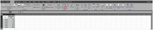
In this case, the independent variable is the year, and the dependent variable is the stock price. Using a chart, the investor can see the changes in the dependent variable in relation to the independent variable. The best chart for this purpose is a scatter chart.

The data must be selected or highlighted to create a scatter chart. From there, the option to create a scatter chart is available under the 'Insert' tab in Excel 2019. It is as below.

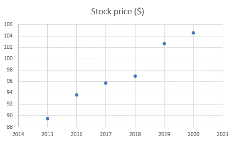
It will produce a chart similar to the one below.

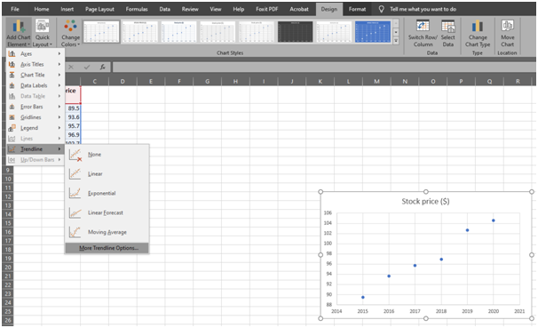
The next step is to generate a trendline. The option to create a trendline is online available if the chart is selected. The trendline option becomes available by selecting the chart and going to the tab and clicking on 'Add chart element'. The easiest way to create a trendline is to use the 'Linear' option from the 'Trendline list'.

However, for Linear Regression, it is critical to click the 'More Trendline Options' option, as shown below.

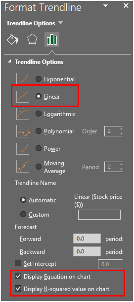
This option will open a new sidebar on the right. By selecting the 'Linear' option from the bar, the chart will display a linear line. From there, the options 'Display Equation on chart' and 'Display R-squared value on chart' will give information related to linear regression, as follows.

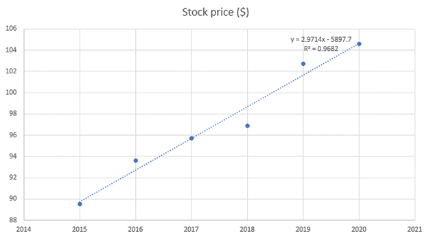
It will give information related to linear regression on the chart. The final chart will look similar to the following.

In the above equation, 'y' signifies the linear regression of the given data. The 'R²' shows the percentage of variance in the dependent variable that the independent variable explains collectively.

Conclusion

Linear regression is a technique used to determine the relationship between two variables. There are some assumptions that investors need to make to use it. The best way to perform linear regression in Excel is through the use of the charts feature, as explained above.

Post Source Here: Linear Regression in Excel