|
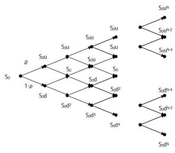
In a previous post, we provided an example of pricing American options using an analytical approximation. Such a pricing model is fast and accurate enough for risk management purposes. However, sometimes more accurate results are required. For this purpose, the binomial (lattice) model can be used. Wikipedia describes the binomial tree model as follows, In finance, the binomial options pricing model (BOPM) provides a generalizable numerical method for the valuation of options. The binomial model was first proposed by Cox, Ross and Rubinstein in 1979. Essentially, the model uses a "discrete-time" (lattice based) model of the varying price over time of the underlying financial instrument... The binomial pricing model traces the evolution of the option's key underlying variables in discrete-time. This is done by means of a binomial lattice (tree), for a number of time steps between the valuation and expiration dates. Each node in the lattice represents a possible price of the underlying at a given point in time. Valuation is performed iteratively, starting at each of the final nodes (those that may be reached at the time of expiration), and then working backwards through the tree towards the first node (valuation date). The value computed at each stage is the value of the option at that point in time.
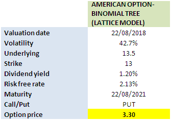
We utilized the lattice model previously to price convertible bonds. In this post, we’re going to use it to value an American equity option. We use the same input parameters as in the previous example. Using our Excel workbook, we obtain a price of $3.30, which is smaller than the price determined by the analytical approximation (Barone-Andesi-Whaley) approach. [caption id="attachment_561" align="aligncenter" width="335"] Click on the link below to download the Excel Workbook. Post Source Here: Valuing an American Option Using Binomial Tree-Derivative Pricing in Excel
0 Comments
R. Merton published a seminal paper [1] that laid the foundation for the development of structural credit risk models. In this post, we’re going to provide an example of how it can be used for managing credit risks. Within the Merton model, equity of a firm is considered a call option on its asset, and it is expressed as follows,
where E denotes the equity of the firm, V is the firm’s asset, B is the notional amount of the debt, r is the risk-free interest rate, and
We note that both asset (V) and its volatility
These 2 equations can be solved simultaneously in order to obtain V and its volatility
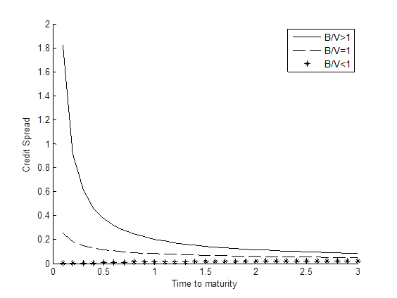
Having the credit spread, we will be able to calculate the probability of default (PD). Loss given default (LGD) can also be derived under Merton framework. Graph below shows the term structures of credit spread under various scenarios for the leverage ratio (B/V). [caption id="attachment_541" align="aligncenter" width="564"] It’s worth mentioning that the Merton model usually underestimates credit spreads. This is due to several factors such as the volatility risk premium, firm’s idiosyncratic risks and the assumptions embedded in the Merton model. This phenomenon is called the credit spread puzzle. Research is being conducted actively in order to improve the model. References [1] Merton, R. C. 1974, On the Pricing of Corporate Debt: The Risk Structure of Interest Rates, Journal of Finance, Vol. 29, pp. 449–470. Article Source Here: Credit Risk Management Using Merton Model |
Archives
April 2023
|


 American option valuation in Excel using Binomial Tree[/caption]
 is the asset volatility,
 are not observable. However, the asset volatility can be related to equity and its volatility through the following equation,
 denotes the volatility of equity.
 which are then used to determine the credit spread
 Term structure of credit spread[/caption]
 RSS Feed
